6. Monte-Carlo DL2 analysis

Applying cuts to the data

The Manager allows you to apply cuts to the data through the Cuts`class, or the `DefaultCuts which contains premade sets of cuts, such as global 0.9 gammaness cut or 70% efficiency cut.

Note that in order to use efficiency based of sensitivity imptimized cuts (therefore energy-dependent cuts), you need to have produced correspondin IRFs and cuts files, with a config file that corresponds to the cuts you require.

There are 3 types of cuts :

Global cuts : these cuts are applied to all the data, and are not energy dependent. CutType.GLOBAL
Energy dependent efficiency cuts : cuts based on target gamma and theta efficiencies, and are energy dependent. CutType.EFFICIENCY_OPTIMIZED
Energy dependent sensitivity cuts : these cuts are optimized for sensitivity, and are energy dependent. CutType.SENSITIVITY_OPTIMIZED

With this, you can create any kind of cuts:

from ctlearn_manager.utils import Cuts, CutType, DefaultCuts

# Global cuts
cuts = Cuts(
    cut_type=CutType.GLOBAL,
    gammaness_cut=0.9,
    # theta_cut=0.4,
)
cuts = DefaultCuts.GH_0_9.value

# Efficiency optimized cuts
cuts = Cuts(
    cut_type=CutType.EFFICIENCY_OPTIMIZED,
    efficiency_gammaness=0.7,
    efficiency_theta=0.7,
)
cuts = DefaultCuts.EFF_70.value

# Sensitivity optimized cuts
cuts = Cuts(cut_type=CutType.SENSITIVITY_OPTIMIZED)

DL2 Visualisation

CTLearn Manager offers a variety of tools to visualize the performance of your model. Below, you will find all the plots thatcan be produced from the DL2 Monte-Carlo files used for testing. They are split in 3 categories: gamma-hadron classification, direction reconstruction, and energy reconstruction. It is good practice to define the zenith and azimuth of your Monte-Carlo files before plotting. They are printed when you load the TriModelManager.

zenith, azimuth = 10 * u.deg, 180 * u.deg

Gamma-Hadron classification

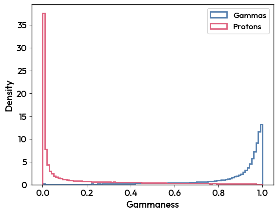
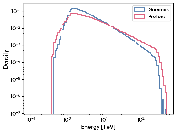
A useful plot for quick checking of the classification performance is the distribution of the classification score for gammas and protons. The ROC curve is also a good way to visualize the performance of the model.

Distribution

Plot the distribution of the classification score for gammas and protons.

Tri_Model.plot_DL2_classification(zenith, azimuth)

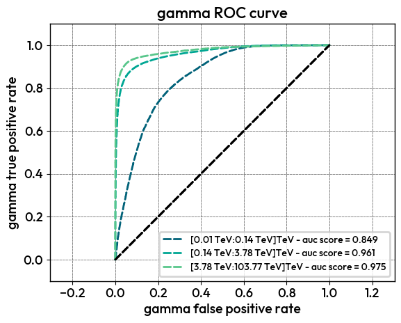
ROC curves

Plot the ROC curve for the gamma-hadron classification, in bins of energy.

Tri_Model.plot_ROC_curve_DL2(zenith, azimuth, nbins=3)

Direction reconstruction

Plot the angular resolution and sky maps of your DL2 data.

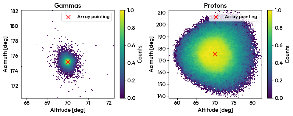
Sky maps

Tri_Model.plot_DL2_AltAz(zenith, azimuth, particle_types=[ParticleType.GAMMA_POINT, ParticleType.PROTON])

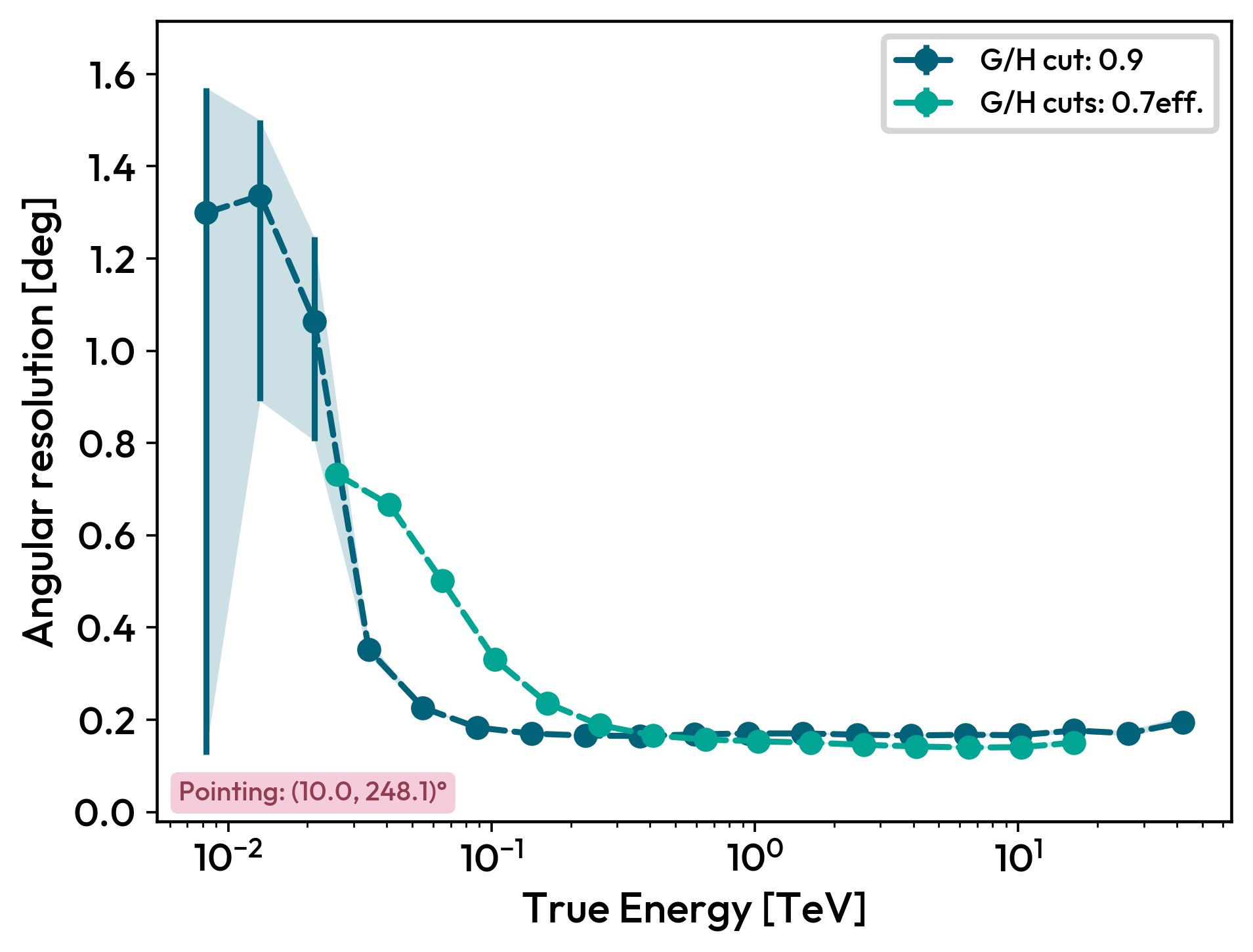
Angular resolution

The angular resolution can be plot for a list of directions, if you leave the zeniths and azimuths empty, the Manager will plot all available directions by default. You can have either mutliple zeniths and azimuths, or multiple cuts. You can also specify the ParticleType to plot the angular resolution for a specific type of particle.

Tri_Model.plot_angular_resolution_DL2([zenith], [azimuth], cuts=[DefaultCuts.EFF_70.value]) # One specific zenith and azimuth with 70% efficiency cut, you can have multiple zeniths and azimuths if you only have one cut
Tri_Model.plot_angular_resolution_DL2([zenith], [azimuth], cuts=[DefaultCuts.EFF_70.value, Cuts(gammaness_cut=0.9)]) # One specific zenith and azimuth with 70% efficiency cut and global 0.9 gammaness cut
Tri_Model.plot_angular_resolution_DL2(cuts=[Cuts(gammaness_cut=0.9)]) # All available zeniths and azimuths with gloabal 0.9 gammaness cut

Energy reconstruction

Plot the energy distribution, migration matrix, and energy resolution of your DL2 data.

Distribution

Tri_Model.plot_DL2_energy(zenith, azimuth)

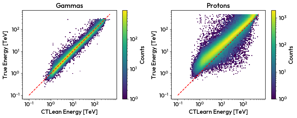
Migration matrix

Specify the desired ParticleType in a list to to plot one migration matrix for each type of particle. .. code-block:: python

Tri_Model.plot_migration_matrix(zenith, azimuth, particle_types=[ParticleType.GAMMA_POINT, ParticleType.PROTON])

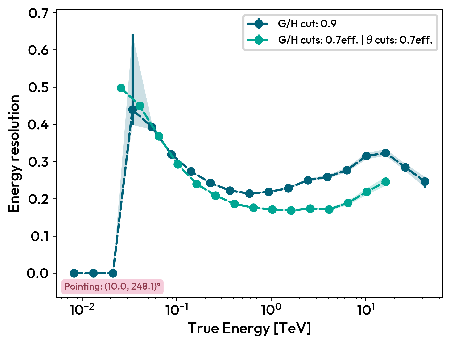
Energy resolution

The energy resolution can be plot for a list of directions, if you leave the zeniths and azimuths empty, the Manager will plot all available directions by default. You can have either mutliple zeniths and azimuths, or multiple cuts. You can also specify the ParticleType to plot the angular resolution for a specific type of particle.

Tri_Model.plot_energy_resolution_DL2([zenith], [azimuth], cuts=[DefaultCuts.EFF_70.value, Cuts(gammaness_cut=0.9)])